Parameter Tuning
In some cases, the default values used in the segmentation process
do not result in the desired results. In this case, the various parameters
that are invovled can be manually set by the user. These parameters are
all defined and available through the seg1d.Segmenter() class.
In this example, the attributes of the segmentation algorithm will be demonstrated through a sine wave with added noise. In this example, the seed used for the random noise is the same in both the target and reference, although a different SNR is used.
First we import seg1d, a helper function for adding noise in the example called
segnoise, and the plotting utils from matplotlib.
>>> import seg1d
>>> import numpy as np
>>> import matplotlib.pylab as plt
>>> import seg1d.examples.noise as segnoise
Next an array of data is generated and a sine wave is created. A signal-noise ratio of 30 is added to the sine wave.
>>> # create an array of data
>>> x = np.linspace(-np.pi*2, np.pi*2, 2000)
>>> # get an array of data from a sin function
>>> targ = np.sin(x)
>>> # add noise to the signal
>>> np.random.seed(123)
>>> targ = segnoise.add_noise(targ,snr=30)
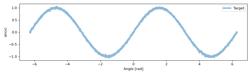
The target data that is used for finding segments in looks like:
>>> # Plot the target
>>> plt.figure(figsize=(10,3))
>>> plt.plot(x, targ,linewidth=4,alpha=0.5,label='Target')
>>> plt.xlabel('Angle [rad]')
>>> plt.ylabel('sin(x)')
>>> plt.legend()
>>> plt.tight_layout()
>>> plt.show()
Now another noisy sine wave is created and a segment of it is cut out.
>>> # define a segment within the sine wave to use as reference
>>> t_s,t_e = 200,400
>>> # number of reference datasets to generate for the example
>>> # make reference data with different random noise on a segment of the original
>>> np.random.seed(123)
>>> refData = segnoise.add_noise(np.sin(x),snr=45)[t_s:t_e]
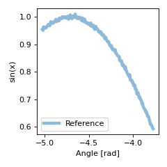
The reference data looks like:
>>> plt.figure(figsize=(3,3))
>>> # Plot the reference
>>> plt.plot(x[t_s:t_e], refData,linewidth=4,alpha=0.5,label='Reference')
>>> plt.xlabel('Angle [rad]')
>>> plt.ylabel('sin(x)')
>>> plt.legend()
>>> plt.tight_layout()
>>> plt.show()
To find the sub-series segment, an instance of the Segmenter class is created,
basic scaling parameters, and the target and reference data are assigned.
>>> # Make an instance of the segmenter
>>> s = seg1d.Segmenter()
>>> #set scaling parameters
>>> s.minW,s.maxW,s.step = 90, 110, 1
>>> #Set target and reference data
>>> s.set_target(targ)
>>> s.add_reference(refData)
>>> #call the segmentation algorithm
>>> segments = s.segment()
>>> np.around(segments, decimals=7)
array([[1.200000e+03, 1.420000e+03, 9.916268e-01],
       [2.000000e+02, 4.000000e+02, 9.904041e-01],
       [4.000000e+02, 5.820000e+02, 8.933443e-01],
       [1.421000e+03, 1.601000e+03, 8.833249e-01]])
After running the segmentation algorithm, we plot the segment the reference data should be located, along with the segments that were found.
>>> plt.figure(figsize=(10,3))
>>> #plot the full sine wave
>>> plt.plot(x, targ,linewidth=4,alpha=0.2,label='Target')
>>> #plot the location of the original reference segment
>>> # NOTE this is just the location, the actual reference data is shown above
>>> plt.plot(x[t_s:t_e], targ[t_s:t_e],linewidth=6,alpha=0.7,label='Reference')
>>> #plot all segments found
>>> seg_num = 1
>>> for seg in segments:
...     st = seg[0]
...     e = seg[1]
...     plt.plot(x[st:e], targ[st:e],dashes=[1,1],linewidth=2,alpha=0.8,
...     label='Segment {}'.format(seg_num))
...     seg_num += 1
>>> plt.xlabel('Angle [rad]')
>>> plt.ylabel('sin(x)')
>>> plt.legend()
>>> plt.tight_layout()
>>> plt.show()
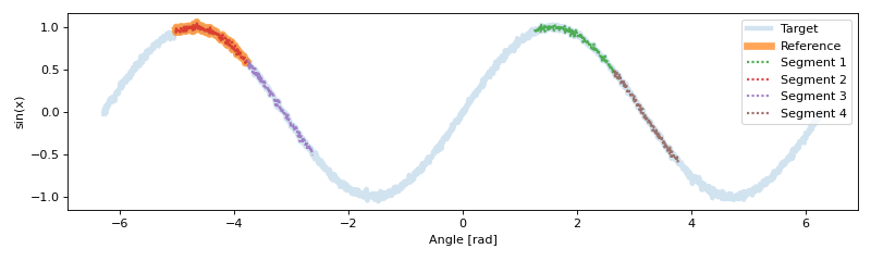
From the plot, it is clear there are segments that do not belong.
By accessing the Segmenter attributes, the algorithm and this error are better understood (and resolved).
>>> # First we look at the original segments before clustering
>>> np.around(s.groups, decimals=7)
array([[1.200000e+03, 1.420000e+03, 9.916268e-01],
       [2.000000e+02, 4.000000e+02, 9.904041e-01],
       [4.000000e+02, 5.820000e+02, 8.933443e-01],
       [1.421000e+03, 1.601000e+03, 8.833249e-01],
       [5.830000e+02, 7.650000e+02, 7.286635e-01],
       [1.602000e+03, 1.782000e+03, 6.541974e-01]])
As shown in the output, there are a total of 6 segments found before clustering.
As the distribution of segments is apporx. [0.99,0.99,0.89,0.88,0.72,0.65],
the attribute, Segmenter.cAdd, (defaults to 0.5) that is added for forcing clusters
only combines the last two values, 0.72 and 0.65 in the lower cluser.
Modifying this attribute would then change the clusters, for example:
>>> s.cAdd = 0.8
>>> np.around(s.segment(), decimals=7)
array([[1.200000e+03, 1.420000e+03, 9.916268e-01],
       [2.000000e+02, 4.000000e+02, 9.904041e-01]])
If the attribute is removed, then only the original segments are used in the clustering.
However, this results in the same cluster as the original where the default of cAdd was 0.5.
>>> s.cAdd = None
>>> np.around(s.segment(), decimals=7)
array([[1.200000e+03, 1.420000e+03, 9.916268e-01],
       [2.000000e+02, 4.000000e+02, 9.904041e-01],
       [4.000000e+02, 5.820000e+02, 8.933443e-01],
       [1.421000e+03, 1.601000e+03, 8.833249e-01]])
Alternatively, the minimum correlation for a given segment can be set with the Segmenter.cMin attribute.
>>> s.cMin = 0.9
>>> np.around(s.segment(),decimals=7)
array([[1.200000e+03, 1.420000e+03, 9.916268e-01]])
Since the cAdd was removed, the only segments available (higher than 0.9 correlation)
were both 0.99, making the clustering result in a single segment.
If cAdd is set back to the default, the segment is correct.
>>> s.cAdd = 0.5
>>> segments = s.segment()
>>> np.around(segments, decimals=7)
array([[1.200000e+03, 1.420000e+03, 9.916268e-01],
       [2.000000e+02, 4.000000e+02, 9.904041e-01]])
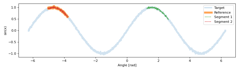
Finally, plotting these segments shows the alignment and logical sub-series identification.
>>> plt.figure(figsize=(10,3))
>>> #plot the full sine wave
>>> plt.plot(x, targ,linewidth=4,alpha=0.2,label='Target')
>>> #plot the original reference segment
>>> plt.plot(x[t_s:t_e], targ[t_s:t_e],linewidth=6,alpha=0.7,label='Reference')
>>> #plot all segments found
>>> seg_num = 1
>>> for seg in segments:
...     st = seg[0]
...     e = seg[1]
...     plt.plot(x[st:e], targ[st:e],dashes=[1,1],linewidth=2,alpha=0.8,
...     label='Segment {}'.format(seg_num))
...     seg_num += 1
>>> plt.xlabel('Angle [rad]')
>>> plt.ylabel('sin(x)')
>>> plt.legend()
>>> plt.tight_layout()
>>> plt.show()