Feature Processing

If there is a series of references that have different lengths, or the weighting is unknown, this example can help guide users to process the data.

In this example we use a few utilities provided by seg1d to process raw data. In many of the other examples, a reference set, target data, and weighting is assumed or provided as sample. If you have data from multiple sources, perhaps of different lengths of time (or samples of points) or varying features, the data must be rescaled and parsed for the matching features. This example also shows how to generate the feature weights, which will compare a set of references and find the features most simliar between them (as a normalized sum of all features).

First we import numpy and matplotlib (to plot for the example)

>>> import numpy as np
>>> import matplotlib.pyplot as plt

Then import the base seg1d and the seg1d processing module

>>> import seg1d
>>> import seg1d.processing as proc

########################## SEG1D Processing #######################

To start, we load an array of dictionaries provided as sample data in seg1d. raw_r is the set of references, and raw_t is a set of targets

>>> raw_r, raw_t = seg1d.sample_input_data()

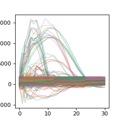
First we can take a look at the reference datasets, noticing they are all different lengths

>>> plt.figure(figsize=(3,3))  
>>> for r in raw_r:
...     plt_r = np.asarray( [ x for x in r.values()  ]  ).T
...     plt.plot(plt_r,alpha=0.3)  
>>> plt.show()  

(Source code)

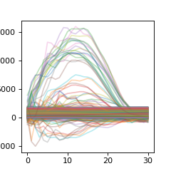
Match feature length and center time series

The first function we use for pre-processing the data is match_len. This will take the largest array of all reference datasets and rescale the other datasets to this longer size

>>> ref_data = proc.Features.match_len(raw_r)

We can now plot the length-matched datasets to see how the reference segments do show similarity over the same scaled timespan

>>> plt_r = np.asarray( [ x for y in ref_data for x in y.values()  ]  ).T
>>> plt.figure(figsize=(3,3))  
>>> plt.plot(plt_r,alpha=0.3)  
>>> plt.show()  

(Source code)

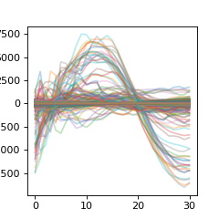
This next process is not always necessary, but is convenient to know. It simply shifts the mean of each array in the references to center along the 0 axis.

>>> ref_data = proc.Features.center(ref_data)

Make sure all reference data has valid keys In this step, we use the shared function by passing all the datasets we will will use to ensure no feature keys are missing. This requires a dictionary to map each feature correctly

>>> ref_data, tar_data = proc.Features.shared(ref_data, raw_t)

Generate weights from the segmented data One of the most important steps for many use cases is the automatic weighting of multiple features. The gen_weights function takes a list of reference datasets and finds the features that match best among all of the references. It then normalizes all the results from 0 to 1. This is important to note, as it means some features will not be used. If all of your features are necessary or should be used, this function should be skipped.

>>> weights = proc.Features.gen_weights(ref_data)

Finally, the last step of pre-processing is to get which params to use and limit to specific ones. In this example, we take only the top 20 features, limit to the normalized score of 0.8, and pass an empty list, which means we use all available features. If there was a list of features that you wanted to include, passing this key list of strings would be possible.

>>> weight_dict = proc.Features.meaningful(weights, limit=0.8, top=20, include_keys=[])

Now we can take a look at the reference data that we will use for segmentation. This data has also been centered (a few steps before)

>>> plt_r = np.asarray( [ x for y in ref_data for x in y.values()  ]  ).T
>>> plt.figure(figsize=(3,3))  
>>> plt.plot(plt_r,alpha=0.3)  
>>> plt.show()  

(Source code)

########################## SEG1D Analysis #######################

At this point the data is properly processed and features weighted. From here on, the normal segmentation process (as seen in the other examples) is applied.

>>> s = seg1d.Segmenter()
>>> s.minW, s.maxW, s.step = 70, 150, 1

>>> for r in ref_data: 
...     s.add_reference(r)

As this sample dataset has multiple targets, we will just use the first one. However, you could iterate over all the target trials by wrapping the remaining code under this example loop: for idx, target in enumerate(tar_data):

Run the analysis on the first target data.

>>> target = tar_data[0]

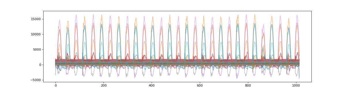
We can visualize this target data before segmentation

>>> plt_t = np.asarray( [ x for x in target.values() ] )
>>> plt.figure(figsize=(15,4))  
>>> plt.plot(plt_t.T,alpha=0.5)  
>>> plt.show()  

(Source code)

>>> s.set_target(target)

>>> s.w = weight_dict
>>> segments = s.segment()
>>> print(np.around(sorted(segments, key=lambda x: x[0])[:3], decimals=5))
[[ 42.       67.        0.99856]
 [112.      137.        0.99864]
 [181.      208.        0.99709]]

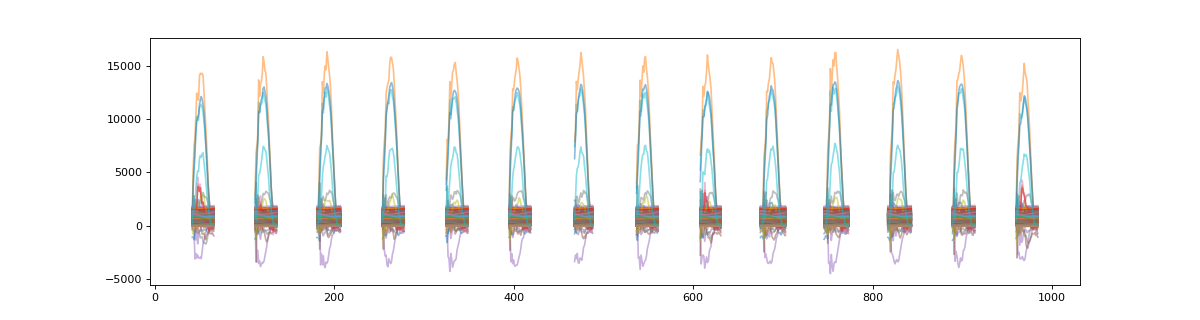
Now that we have segmented the data, the masked array can be plotted to show the results.

>>> plt_t = s.t_masked #get a NaN masked array of the target data
>>> # plot masked target
>>> plt.figure(figsize=(15,4))  
>>> plt.plot(plt_t.T,alpha=0.5)  
>>> plt.show()  

(Source code)