Visualize a Path

Overview

This example uses a simple obj file included in example models. For context of what the top-down view is based on, see the figure below.

Start with the required imports

>>> import matplotlib.pyplot as plt
>>> import numpy as np
>>>
>>> import dhart
>>> from dhart.geometry import LoadOBJ
>>> from dhart.graphgenerator import GenerateGraph
>>> from dhart.raytracer import EmbreeBVH
>>> from dhart.pathfinding import DijkstraShortestPath

Next, load a model and create the BVH

>>> # Get a sample model path
>>> obj_path = dhart.get_sample_model("energy_blob_zup.obj")
>>>
>>> # Load the obj file
>>> obj = LoadOBJ(obj_path)
>>>
>>> # Create a BVH
>>> bvh = EmbreeBVH(obj, True)

Now set parameters to be used for the graph generator. First, we will use a large step size which will ignore any small bumps in the mesh. Later on we will compare the resulting graphs.

>>> # Set the graph parameters
>>> start_point = (-30, 0, 20)
>>> spacing = (1, 1, 10)
>>> max_nodes = 5000
>>> up_step, down_step = 5, 5
>>> up_slope, down_slope = 60, 60
>>> max_step_connections = 1
>>>
>>> # Generate the Graph
>>> graph = GenerateGraph(bvh, start_point, spacing, max_nodes,
...                         up_step,up_slope,down_step,down_slope,
...                         max_step_connections, cores=-1)
>>>
>>> # Get Nodes
>>> nodes = graph.getNodes()
>>> print(f"Graph Generated with {len(nodes.array)} nodes")
Graph Generated with 3450 nodes

Once the graph is generated, we can define an array of spatial points and get the closest nodes of the graph to these points.

>>> # Define a start and end point in x,y
>>> p_desired = np.array([[-30,0],[30,0]])
>>> closest_nodes = graph.get_closest_nodes(p_desired,z=False)
>>> print("Closest Node: ", closest_nodes)
Closest Node:  [   0 3123]
>>>
>>> # Define a start and end node to use for the path (from, to)
>>> start_id, end_id = closest_nodes[0], closest_nodes[1]

Now we call the shortest path algorithm on the default cost, which is euclidean distance. We can take the sum of the cost values in the array and print it to use as a comparison later.

>>> # Call the shortest path
>>> path = DijkstraShortestPath(graph, start_id, end_id)
>>>
>>> # As the cost array is numpy, simple operations to sum the total cost can be calculated
>>> path_sum = np.sum(path['cost_to_next'])
>>> print('Total path cost: ', path_sum)
Total path cost:  62.035927

>>> # Get the x,y,z values of the nodes at the given path ids
>>> path_xyz = np.take(nodes[['x','y','z']], path['id'])
>>>
>>> # Extract the xyz locations of the nodes
>>> x_nodes, y_nodes, z_nodes = nodes['x'], nodes['y'], nodes['z']
>>>
>>> # Extract the xyz locations of the path nodes
>>> x_path, y_path, z_path = path_xyz['x'], path_xyz['y'], path_xyz['z']
>>>
>>> # Plot the graph
>>> plt.scatter(x_nodes, y_nodes, c=z_nodes, alpha=0.5) 
>>> plt.plot(x_path,y_path, c="red", marker='.',linewidth=3) 
>>> plt.show() 

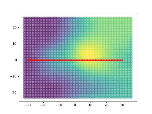
As seen in the image, the shortest path on this graph is a straight line.

(Source code)

Repeat the process with a new graph based on different parameters and same locations We change the graph parameters to limit a ‘step’.

>>> # Change some graph parameters
>>> up_step, down_step = 0.2, 0.5
>>>
>>> # Generate a new Graph
>>> graph = GenerateGraph(bvh, start_point, spacing, max_nodes,
...                         up_step,up_slope,down_step,down_slope,
...                         max_step_connections, cores=-1)

We now get the nodes of the new graph, and can see the number of nodes are the same.

>>> nodes = graph.getNodes()
>>> print(f"Graph Generated with {len(nodes.array)} nodes")
Graph Generated with 3450 nodes

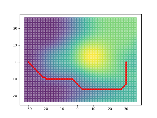
If we now get the closest node, it is now a different index. The key here is that the limitations of the graph generator step size have caused certain edges to not be valid, which changed the order in which nodes were created.

>>> closest_nodes = graph.get_closest_nodes(p_desired,z=False)
>>> print("Closest Node: ", closest_nodes)
Closest Node:  [   0 2597]
>>>
>>> start_id, end_id = closest_nodes[0], closest_nodes[1]
>>> path = DijkstraShortestPath(graph, start_id, end_id)

If we sum the costs of the path, we see it has now increased. Important to note, we did not change the cost type when querying the shortest path. Instead, it is the lack of edge connections due to the graph generator settings. While the total number of nodes are the same, there a missing edges, which forces the shortest path by distance to travel around the thresholds defined when creating the graph.

>>> # As the cost array is numpy, simple operations to sum the total cost can be calculated
>>> path_sum = np.sum(path['cost_to_next'])
>>> print('Total path cost: ', path_sum)
Total path cost:  81.40916

Now extract the location data for the nodes and path to be plotted.

>>> path_xyz = np.take(nodes[['x','y','z']], path['id'])
>>> x_nodes, y_nodes, z_nodes = nodes['x'], nodes['y'], nodes['z']
>>> x_path, y_path, z_path = path_xyz['x'], path_xyz['y'], path_xyz['z']
>>>
>>> # Plot the graph
>>> plt.scatter(x_nodes, y_nodes, c=z_nodes, alpha=0.5) 
>>> plt.plot(x_path,y_path, c="red", marker='.',linewidth=3) 
>>> plt.show() 

Seen in the image, the path avoids the center mound as it was too steep for the graph generator to run on.

(Source code)