Visualize the Graph¶

Overview¶

This example uses a simple obj file included in example models. For context of what the top-down view is based on, see the figure below.

Basic Graph Visualization¶

import matplotlib.pyplot as plt
from mpl_toolkits.mplot3d import Axes3D

from dhart.geometry import LoadOBJ
from dhart.raytracer import EmbreeBVH
from dhart.graphgenerator import GenerateGraph
import dhart

# Get a sample model path
obj_path = dhart.get_sample_model("energy_blob_zup.obj")

# Load the obj file
obj = LoadOBJ(obj_path)

# Create a BVH
bvh = EmbreeBVH(obj, True)

# Set the graph parameters
start_point = (0, -20, 20)
spacing = (1, 1, 10)
max_nodes = 5000
up_step, down_step = 0.5, 0.5
up_slope, down_slope = 20, 20
max_step_connections = 1

# Generate the Graph
graph = GenerateGraph(bvh, start_point, spacing, max_nodes,
                        up_step,up_slope,down_step,down_slope,
                        max_step_connections, cores=-1)

# Convert the graph to a CSR
csr_graph = graph.CompressToCSR()

# Get the nodes of the graph as a list of x,y,z,type,id tuples
nodes = graph.getNodes()

# get the x,y,z coordinates of the nodes
x = [ n[0] for n in nodes ] # x coordinate
y = [ n[1] for n in nodes ] # y coordinate
z = [ n[2] for n in nodes ] # z coordinate

(Source code)

The graph can be plotted in 3D for illustrative purposes (although it is better to load an obj or use a proper engine like OpenGL).

# Plot the graph in 3D
fig = plt.figure()
ax = Axes3D(fig)
ax.view_init(azim=-123, elev=15)

ax.scatter(x, y, z)
plt.show()

(Source code)

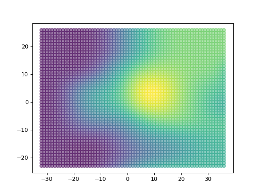
From the top view, this can be plotted in x,y and color nodes by the z value

# Plot the graph
plt.scatter(x, y, c=z, alpha=0.5)
plt.show()

(Source code)

Slope Settings¶

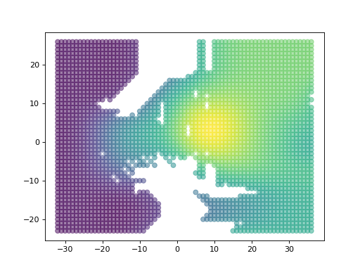
To illustrate the thresholds of this wavy hill, we can reduce the slope tolerances and plot a new graph which shows certain areas are not reachable.

import matplotlib.pyplot as plt

from dhart.geometry import LoadOBJ
from dhart.raytracer import EmbreeBVH
from dhart.graphgenerator import GenerateGraph
import dhart

# Get a sample model path
obj_path = dhart.get_sample_model("energy_blob_zup.obj")
print(obj_path)

# Load the obj file
obj = LoadOBJ(obj_path)

# Create a BVH
bvh = EmbreeBVH(obj, True)

# Set the graph parameters
start_point = (0, 0, 20)
spacing = (1, 1, 1)
max_nodes = 5000
up_step, down_step = 0.5, 0.5

max_step_connections = 1

# Set a smaller threshold for slope
up_slope, down_slope = 5, 5

# Add a minimum out-degree for each node

# Generate the Graph
graph = GenerateGraph(bvh, start_point, spacing, max_nodes,
                        up_step,up_slope,down_step,down_slope,
                        max_step_connections, cores=-1)

# Convert the graph to a CSR
csr_graph = graph.CompressToCSR()

# Get the nodes of the graph as a list of x,y,z,type,id tuples
nodes = graph.getNodes()

# get the x,y,z coordinates of the nodes and set the color to the z value
x = [ n[0] for n in nodes ] # x coordinate
y = [ n[1] for n in nodes ] # y coordinate
z = [ n[2] for n in nodes ] # z coordinate

# Plot the graph
plt.scatter(x, y, c=z, alpha=0.5)
plt.show()

(Source code)

Determining Minimum Connections¶

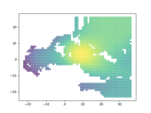
Using the min_connections parameter we can ensure nodes have a minimum number of out directions (out-degree), which can avoid walls/edges and prevent ‘islands’ caused by single edge connections

import matplotlib.pyplot as plt

from dhart.geometry import LoadOBJ
from dhart.raytracer import EmbreeBVH
from dhart.graphgenerator import GenerateGraph
import dhart

# Get a sample model path
obj_path = dhart.get_sample_model("energy_blob_zup.obj")
print(obj_path)

# Load the obj file
obj = LoadOBJ(obj_path)

# Create a BVH
bvh = EmbreeBVH(obj, True)

# Set the graph parameters
start_point = (0, 0, 20)
spacing = (1, 1, 1)
max_nodes = 5000
up_step, down_step = 0.5, 0.5

max_step_connections = 1

# Set a smaller threshold for slope
up_slope, down_slope = 5, 5

# Add a minimum out-degree for each node
min_connections = 3

# Generate the Graph
graph = GenerateGraph(bvh, start_point, spacing, max_nodes,
                        up_step,up_slope,down_step,down_slope,
                        max_step_connections, min_connections, cores=-1)

# Convert the graph to a CSR
csr_graph = graph.CompressToCSR()

# Get the nodes of the graph as a list of x,y,z,type,id tuples
nodes = graph.getNodes()

# get the x,y,z coordinates of the nodes and set the color to the z value
x = [ n[0] for n in nodes ] # x coordinate
y = [ n[1] for n in nodes ] # y coordinate
z = [ n[2] for n in nodes ] # z coordinate

# Plot the graph
plt.scatter(x, y, c=z, alpha=0.5)
plt.show()