Getting Started

In this section, a few simple examples are given to ensure the installation is working and you are able to segment data. These examples call a method provided that uses default parameters for the algorithms within the segmentation process but allows user input for the data related parameters such as scaling and step size for the matching process.

Sample Data

A basic example of checking the installation using the included sample data.

Example using included sample data

>>> import seg1d 
>>> import numpy as np
>>> #retrieve the sample reference, target, and weight data
>>> r,t,w = seg1d.sampleData()
>>> ### define some test parameters
>>> minW = 70 #minimum percent to scale down reference data
>>> maxW = 150 #maximum percent to scale up reference data
>>> step = 1 #step to use for correlating reference to target data
>>> #call the segmentation algorithm
>>> np.around( seg1d.segment_data(r,t,w,minW,maxW,step) , decimals=7 )
array([[207.       , 240.       ,   0.9124224],
       [342.       , 381.       ,   0.8801901],
       [ 72.       , 112.       ,   0.8776795]])

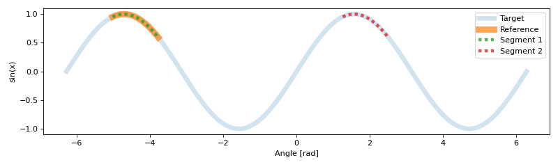
Sine Wave

Sample using sine wave

>>> import seg1d
>>> import numpy as np
>>> import matplotlib.pylab as plt

Data can be constructed as a numpy array

>>> # create an array of data
>>> x = np.linspace(-np.pi*2, np.pi*2, 2000)
>>> # get an array of data from a sin function 
>>> targ = np.sin(x)

To use the basic method interface, the data must be labeled

>>> # define a segment within the sine wave to use as reference
>>> t_s,t_e = 200,400
>>> # cut a segment out to use as a reference data
>>> refData = [ { '0' : targ[t_s:t_e] } ]
>>> targData = {'0' : targ} 
>>> refWeights = {'0' : 1}
>>> 
>>> ### define some test parameters
>>> minWin = 98 #minimum percent to scale down reference data
>>> maxWin = 105 #maximum percent to scale up reference data
>>> sizeStep = 1 #step to use for correlating reference to target data
>>> 
>>> #call the segmentation algorithm
>>> segments = seg1d.segment_data(refData,targData,refWeights,minWin,maxWin,sizeStep)
>>> np.around(segments, decimals=7)
array([[2.000000e+02, 4.000000e+02, 1.000000e+00],
       [1.200000e+03, 1.398000e+03, 9.999999e-01]])

Using matplotlib we can visualize the results

>>> plt.figure(figsize=(10,3)) 
>>> # plot the full sine wave
>>> plt.plot(x, targ,linewidth=6,alpha=0.2,label='Target') 
>>> # plot the original reference segment
>>> plt.plot(x[t_s:t_e], targ[t_s:t_e],linewidth=8,alpha=0.7,label='Reference') 
>>>
>>> # plot all segments found
>>> seg_num = 1
>>> for s,e,c in segments:
...     plt.plot(x[s:e], targ[s:e],dashes=[1,1],linewidth=4,alpha=0.8, 
...     label='Segment {}'.format(seg_num)) 
...     seg_num += 1 
>>> plt.xlabel('Angle [rad]') 
>>> plt.ylabel('sin(x)') 
>>> plt.legend() 
>>> plt.tight_layout() 
>>> plt.show() 

(Source code)

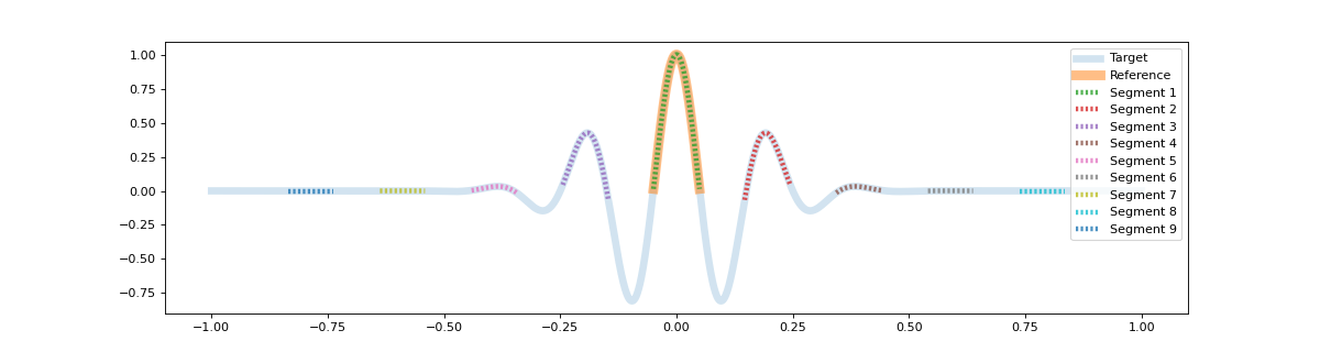
Gauss

In this example a Gaussian pulse is used to show segmentation on the varying shape of different amplitude. As the center arc is given as reference, the multiple extending arcs are found as well. Through the output of the segments, the correlation values can be seen to decrease, although still clustered within the group.

>>> import seg1d 
>>> import numpy as np
>>> import matplotlib.pylab as plt
>>> import scipy.signal as signal 

>>> # create an array of data
>>> x = np.linspace(-1, 1, 2000)
>>> # get an array of data from a Gaussian pulse 
>>> targ = signal.gausspulse(x, fc=5)

>>> # define a segment within the sine wave to use as reference
>>> t_s,t_e    = 950,1050
>>> # cut a segment out to use as a reference data
>>> refData    = [ { 'gauss' : targ[t_s:t_e] } ]
>>> targData   =   { 'gauss' : targ } 
>>> refWeights =   { 'gauss' : 1 }

>>> ### define some test parameters
>>> minWin   = 98 #minimum percent to scale down reference data
>>> maxWin   = 105 #maximum percent to scale up reference data
>>> sizeStep = 1 #step to use for correlating reference to target data

>>> # call the segmentation algorithm
>>> segments = seg1d.segment_data(refData,targData,refWeights,minWin,maxWin,sizeStep)
>>> print(np.around(segments,decimals=7))
[[9.500000e+02 1.050000e+03 1.000000e+00]
 [1.146000e+03 1.245000e+03 9.867665e-01]
 [7.550000e+02 8.540000e+02 9.867665e-01]
 [1.343000e+03 1.441000e+03 9.498135e-01]
 [5.590000e+02 6.570000e+02 9.498135e-01]
 [1.540000e+03 1.638000e+03 8.949109e-01]
 [3.620000e+02 4.600000e+02 8.949109e-01]
 [1.738000e+03 1.836000e+03 8.301899e-01]
 [1.640000e+02 2.620000e+02 8.301899e-01]]

>>> plt.figure(figsize=(15,4)) 
>>> # plot the full pulse
>>> plt.plot(x, targ,linewidth=6,alpha=0.2,label='Target') 
>>> # plot the original reference segment
>>> plt.plot(x[t_s:t_e], targ[t_s:t_e],linewidth=8,alpha=0.5,label='Reference') 
>>> # plot all segments found
>>> seg_num = 1
>>> for s,e,c in segments:
...     plt.plot(x[s:e], targ[s:e],dashes=[0.5,0.5],linewidth=4,alpha=0.8, 
...     label='Segment {}'.format(seg_num)) 
...     seg_num += 1 
>>> plt.legend() 
>>> plt.show() 

(Source code)