ECG

In this example we use the ECG data included with scipy signal module. The references roughly includes the Q-T interval (https://en.wikipedia.org/wiki/Electrocardiography). In the first portion, two sample segments are used. While the segments are not aligned, they are able to find some segments correctly. In the second portion of the example, only one segment is used for the reference data.

>>> import random
>>> import numpy as np
>>> from scipy.misc import electrocardiogram
>>> import matplotlib.pyplot as plt
>>> import seg1d 

After imports, the scipy signal ECG data is called and some segments are taken.

>>> ecg = electrocardiogram() #get the scipy sample data 
>>> ref_slices = [[927, 1057],[1111, 1229]] #pick sample endpoints

>>> s = seg1d.Segmenter()  #create the segmenter

>>> refs = [ ecg[x[0]:x[1]] for x in ref_slices ]
>>> for r in refs: s.add_reference(r) #set reference data

>>> s.set_target(ecg[1500:3500]) #set the target data to the ecg after ref
>>> segments = s.segment()  # run segmenter with defaults

>>> print(np.around(segments,decimals=7))
[[1.607000e+03 1.729000e+03 8.169533e-01]
 [7.380000e+02 8.220000e+02 8.123868e-01]
 [9.190000e+02 1.003000e+03 8.120505e-01]
 [1.439000e+03 1.552000e+03 8.092366e-01]
 [3.600000e+02 4.930000e+02 8.077664e-01]
 [1.091000e+03 1.213000e+03 8.043364e-01]
 [1.775000e+03 1.895000e+03 7.998723e-01]
 [1.720000e+02 3.000000e+02 7.926582e-01]
 [1.268000e+03 1.340000e+03 7.847107e-01]
 [5.540000e+02 6.280000e+02 7.802931e-01]]

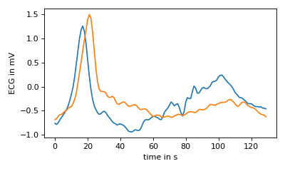
The reference data is automatically scaled to the largest reference in the dataset when the segment method is called. Therefore, by retrieving this attribute we can plot what the reference set looks like when the lengths are normalized.

In the example, it is clear the peaks of the reference segments are not aligned. This discrepency, due to the averaging of all reference data items, will be seen in the final segments of the target data later.

>>> refs = s.r
>>> refs = np.asarray( [ x[y] for x in refs for y in x ] )

>>> plt.figure(figsize=(5,3))  
>>> plt.plot(refs.T)  
>>> plt.xlabel("time in s")  
>>> plt.ylabel("ECG in mV")  
>>> plt.tight_layout()  
>>> plt.show()  

(Source code)

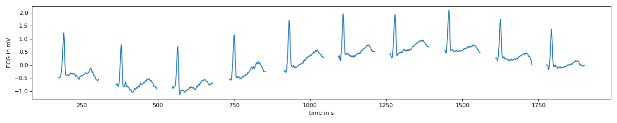
The final segments are shown by calling the property t_masked which returns the target data as an ndarray with NaN values for areas not found to be segments.

>>> plt.figure(figsize=(15,3))  
>>> plt.plot(s.t_masked.T)  
>>> plt.xlabel("time in s")  
>>> plt.ylabel("ECG in mV")  
>>> plt.tight_layout()  
>>> plt.show()  

(Source code)

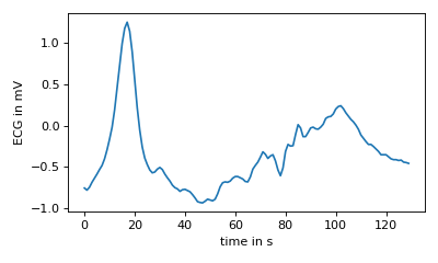
>>> #use only 1 reference
>>> s.clear_reference()
>>> s.add_reference( ecg[927:1057] )

>>> refs = s.r
>>> refs = np.asarray( [ x[y] for x in refs for y in x ] )

>>> plt.figure(figsize=(5,3))  
>>> plt.plot(refs.T)  
>>> plt.xlabel("time in s")  
>>> plt.ylabel("ECG in mV")  
>>> plt.tight_layout()  
>>> plt.show()  

(Source code)

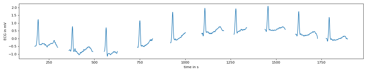
>>> #remove first part of data (contains reference)
>>> s.set_target(ecg[1500:3500])
>>> s.nC = 2
>>> s.cMin = 0.7

>>> segments = s.segment()

>>> print(np.around(segments,decimals=7))
[[7.350000e+02 8.540000e+02 9.462850e-01]
 [1.093000e+03 1.213000e+03 9.242974e-01]
 [9.140000e+02 1.046000e+03 9.059727e-01]
 [3.620000e+02 4.980000e+02 9.009127e-01]
 [5.470000e+02 6.800000e+02 8.940106e-01]
 [1.262000e+03 1.390000e+03 8.868629e-01]
 [1.776000e+03 1.902000e+03 8.771139e-01]
 [1.609000e+03 1.729000e+03 8.689476e-01]
 [1.440000e+03 1.559000e+03 8.646669e-01]
 [1.730000e+02 3.060000e+02 8.029426e-01]]

>>> res = s.t_masked

>>> plt.figure(figsize=(15,3))  
>>> plt.plot(res.T)  
>>> plt.xlabel("time in s")  
>>> plt.ylabel("ECG in mV")  
>>> plt.tight_layout()  
>>> plt.show()  

(Source code)